Monday, January 5, 2015

Comparing Apache Avro to Protocol Buffers, XML and JSON payloads

Comparing Avro to Protocol Buffers, XML and JSON payloads

In a previous blog post I compared Mainframe COBOL payloads to Protocol Buffers, XML and JSON.

The idea was to compare the number of bytes needed to encode structured data in these various languages.

The results were:

LanguageBytes size
Mainframe 422
XML1960
JSON1275
Protobuf 403

Since we have recently introduced legstar support for Apache Avro, I was curious to get a sense of how optimized Avro is. So I performed the same test and came out with 370 bytes.

Of course, you will get different results with different COBOL structures and a different data mix but you can be practically sure you will get a smaller Avro payload than the Mainframe payload.

This is because a lot of optimization has gone into the Avro binary encoder (testing was done using Avro 1.7.7).

Taking the same example as in the previous blog post, with this COBOL structure:

05 QUERY-DATA.
              10 CUSTOMER-NAME               PIC X(20).
              10 MAX-REPLIES                 PIC S9(4) COMP VALUE -1.

these 22 bytes of mainframe data :
0xe25c4040404040404040404040404040404040400005

gets translated to just 4 Avro bytes:
0x04532A0A

The corresponding Avro schema being:
{
      "type":"record",
      "name":"QueryData",
      "fields":[{
          "name":"customerName",
          "type":"string"
        },
        {
          "name":"maxReplies",
          "type":"int"
        }
      ],
      "namespace":"com.legstar.avro.samples.lsfileaq"
    }

This is interesting because it means that if you take a large mainframe file and convert it to Avro, you are likely to get a smaller file. About 12% smaller in the particular case used in my testing.

If you are using Hadoop, and have a use case where the same mainframe file is read by several MapReduce jobs, then it could make sense to convert your mainframe file using legstar.avro before you store it in HDFS as Avro encoded.

Reading that file later will be faster as the volume of data read off HDFS will be smaller.

Tuesday, December 9, 2014

LegStar V2 is underway

LegStar has been around for a while now, 8 years since the first release in 2006.

Since then a lot of things have changed:

  • The java SDK is now in version 8. It was version 4 in 2006 and things like generics were unheard of
  • Programming patterns have become common practice
  • Multi-threading techniques have improved and are better understood
  • Use cases which used to be centered around remote procedure calls to CICS programs, now deal with massive imports of mainframe data for Big Data Analytics


Some parts of LegStar are showing their age and I have finally found some time to start rewriting some of the core features. The LegStar core project is the older in the product so this is where I started.

The legstar-core2 project is where I placed the new developments.

You should not consider this as a replacement to the current LegStar though:

  • There are far less functionalities in legstar-core2 at the moment than in LegStar
  • The API V2 will not be backward compatible 


That second point may come as a surprise for mainframe users but in the world of open source, breaking compatibility is an "art de vivre". A primary benefit is that the code you get is much cleaner and readable when it does not need to deal with legacy. When the project evolves though, we might want to work on a migration guide of some form.

The new legstar-core2 project contains a simplified version of the legstar-cob2xsd module which is the venerable COBOL to XML schema translator. The changes are minor in this module so far. Neither COBOL, nor the XML schema specs have changed much.

From an architecture standpoint the major change is that JAXB is no longer central to the conversion process. So far, we were always going through the JAXB layer even if the target was Talend, Pentaho, JSON, or any other format.

Now the conversion logic has been abstracted out in a legstar-base module. There is also an associated legstar-base-generator module that produces artifacts for legstar-base. The legstar-base module can be considered a complete low-level solution for mainframe to java conversions. This new legstar-base module has replaced the legstar-coxbapi and legstar-coxbrt modules.

JAXB is still supported of course with 2 new modules, legstar-jaxb and legstar-jaxb-generator which cover the old legstar-coxbgen features.

Besides the architectural changes, there are 2 important changes you need to be aware of:

  • The legstar-core2 project is hosted on Github, not on Google code. Therefore source control has moved from SVN to Git.
  • The licence is GNU Affero GPL which is not as business friendly as the LGPL used by LegStar


Again, this is just the beginning on this new project and its likely to make its way to the newest developments first (such as legstar-avro). Over time, I will describe the new features in more details. In the meanwhile please send any feedback.

Fady

Friday, November 7, 2014

Announcing LegStar for Apache Avro

legStar has dealt with mapping COBOL structures to other languages for a long time now. Such a mapping has not always been straightforward because COBOL has a number of constructs that sets it appart, namely:

  • Deep hierarchies. Structures in COBOL tend to be several levels deep with the parent hierarchy providing a namespace system (the same field name can appear in several places in a structure).
  • Variable size arrays (Arrays whose dimension is given at runtime by another field in the structure).
  • Redefines which are similar to C unions.
  • Decimal data types which have a fixed number of digits in the fractional part (fractions whose denominator is a power of ten). I am surprised at how many languages try to get away with double/float as the only way to represent fractions.

Data serialization and RPC

Over the last few years, a series of new data serializing languages for structures have appeared. These derive mainly from the need to perform fast Remote Procedure Calls (RPC) over a network with complex data being passed back and forth. For high frequency calls, XML or JSON would be too expensive.

The RPC serializing languages I came across recently are:

Protocol Buffers (PB) was one for which we developed a LegStar translator which was an interesting experience.

Data serialization and Big Data Analytics

Besides RPC, the Big Data Analytics domain is now generating the need for efficient data serialization as well.

One aspect of dealing with large amounts of data is that you need to process records as fast as possible. Traditionally, in the Business Intelligence domain, data was serialized as SQL records or CSV (comma separated) records.

Not suprisingly all first generation ETL tools dealt primarily with SQL and CSV records.

The problem is that SQL and CSV are very bad at storing complex, structured data. Particularly deep hierarchies, arrays and unions.

So when your Big Data is made of such structured data (for instance data originating from a Mainframe), traditional ETL tools are generally sub optimal.

Apache Hadoop, a popular Big Data system, does not impose SQL or CSV. It offers a native serialization mechanism called Writable which allows passing structured data efficiently between Map and Reduce jobs.

Even better, there is an alternative approach called Apache Avro which is a standalone project similar to Protocol Buffers or Thrift but tightly integrated into Hadoop.

Importing Mainframe data into Hadoop

In a scenario where you need to import very large volumes of data from a Mainframe and perform analytics on them, it would make sense to use the Avro format to pass the records between the various steps of the analytics process (Map and Reduce jobs in Hadoop parlance).

The reason is that Mainframe records, described by a COBOL copybook, can translate to Avro records while preserving the hierarchy, arrays and redefines. This saves a lot of processing otherwise needed to 'flatten' the COBOL structures to a columnar representation (SQL, CSV, ...).

What is left to be done is a COBOL to Avro Translator so I have started a new legstar.avro project.

It is an early phase for the project of course and I intend to decribe it further in future installements of this blog. So if you are interested, please stay tuned.

Monday, June 18, 2012

Comparing Protocol Buffers to XML and JSON payloads

Following up on my last blog entry, I was interested in getting some figures comparing payload sizes for data encoded using protocol buffers against XML and JSON.

Since the major argument in favor of protocol buffers is the reduced network impact, I thought it would be interesting to measure that in a mainframe integration environment.

I built my test scenario with a CICS program called LSFILEAQ. LSFILEAQ is part of the legstar test programs and uses a VSAM file that comes with an IBM demo application commonly found in CICS development partitions.

LSFILEAQ takes simple query parameters on input and sends back an array of replies. This is the COBOL structure that describes the LSFILEAQ commarea (its CICS communication area):

        01 DFHCOMMAREA.
           05 QUERY-DATA.
              10 CUSTOMER-NAME               PIC X(20).
              10 MAX-REPLIES                 PIC S9(4) COMP VALUE -1.
                  88 UNLIMITED     VALUE -1.
           05 REPLY-DATA.
              10 REPLY-COUNT                 PIC 9(8) COMP-3.
              10 CUSTOMER OCCURS 1 TO 100 DEPENDING ON REPLY-COUNT.
                  15 CUSTOMER-ID             PIC 9(6).
                  15 PERSONAL-DATA.
                     20 CUSTOMER-NAME        PIC X(20).
                     20 CUSTOMER-ADDRESS     PIC X(20).
                     20 CUSTOMER-PHONE       PIC X(8).
                  15 LAST-TRANS-DATE         PIC X(8).
                  15 FILLER REDEFINES LAST-TRANS-DATE.
                     20 LAST-TRANS-DAY       PIC X(2).
                     20 FILLER               PIC X.
                     20 LAST-TRANS-MONTH     PIC X(2).
                     20 FILLER               PIC X.
                     20 LAST-TRANS-YEAR      PIC X(2).
                  15 LAST-TRANS-AMOUNT       PIC $9999.99.
                  15 LAST-TRANS-COMMENT      PIC X(9).

I ran the program using a query yielding a result of 5 customers and measured the raw size of the commarea in bytes. I came up with 422 bytes. Note that this includes both the input and output parameters. These are untranslated bytes, in z/OS format.

Using the legstar transformers I than generated XML and JSON representations of that same z/OS data. This time, the data is translated to ASCII and formatted using XML or JSON. I than measured the sizes of the corresponding XML and JSON payloads and got:

XML:1960 bytes
JSON:1275 bytes

What these results mean is that if I choose to send XML to CICS instead of the raw z/OS data, I will increase the network load by a factor of 364% (almost 5 times to raw data payload).

If I select the less greedy JSON to encode the payload, the network load increases by 202% (3 times the raw payload).

Now, what would be the equivalent protocol buffers payload?

To answer that, I first wrote a protocol buffer "proto" file using the protocol's Interface Description Language:

package customers;
option java_package = "com.example.customers";
option java_outer_classname = "CustomersProtos";

message CustomersQuery {
  required string customer_name_pattern = 1;
  optional int32 max_replies = 2;
}

message CustomersQueryReply {
  repeated Customer customers = 1;

  message Customer {
    required int32 customer_id = 1;
    required PersonalData personal_data= 2;
    optional TransactionDate last_transaction_date = 3;
    optional double last_transaction_amount = 4;
    optional string last_transaction_comment = 5;

    message PersonalData {
      required string customer_name = 1;
      required string customer_address = 2;
      required string customer_phone = 3;
    }

    message TransactionDate {
      required int32 transaction_year = 1;
      required int32 transaction_month = 2;
      required int32 transaction_day = 3;
    }
  }
}

This is close to the target LSFILEAQ commarea structure.

I then used protobuf-cobol to generate COBOL parsers and writers for each of the protocol buffers messages.

Rather than using the command line generation utility though, I used simple java code that looks like this:

HasMaxSize maxSizeProvider = new HasMaxSize() {

    public Integer getMaxSize(String fieldName, Type fieldType) {
        if (fieldName.equals("customer_name_pattern")) {
            return 20;
        } else if (fieldName.equals("customer_name")) {
            return 20;
        } else if (fieldName.equals("customer_address")) {
            return 20;
        } else if (fieldName.equals("customer_phone")) {
            return 8;
        } else if (fieldName.equals("last_transaction_comment")) {
            return 9;
        }
        return null;
    }

    public Integer getMaxOccurs(String fieldName,
                                JavaType fieldType) {
        if (fieldName.equals("Customer")) {
            return 1000;
        }
        return null;
    }

};
new ProtoCobol()
  .setOutputDir(new File("target/generated-test-sources/cobol"))
  .setQualifiedClassName("com.example.customers.CustomersProtos")
  .addSizeProvider(maxSizeProvider)
  .run();

The "HasMaxSize" provider allows the generated COBOL code to implement the size limitations which are specific to COBOL.

Besides the parsers and writers, protobuf-cobol also generates copybooks for the various messages. This is what we get for the input and output messages:

01  CustomersQuery.
           03  customer-name-pattern    PIC X(20) DISPLAY.
           03  max-replies PIC S9(9) COMP-5.

       01  CustomersQueryReply.
           03  OCCURS-COUNTERS--C.
             05  Customer--C PIC 9(9) COMP-5.
           03  Customer OCCURS 0 TO 1000 DEPENDING ON Customer--C.
             05  customer-id PIC S9(9) COMP-5.
             05  PersonalData.
               07  customer-name PIC X(20) DISPLAY.
               07  customer-address PIC X(20) DISPLAY.
               07  customer-phone PIC X(8) DISPLAY.
             05  TransactionDate.
               07  transaction-year PIC S9(9) COMP-5.
               07  transaction-month PIC S9(9) COMP-5.
               07  transaction-day PIC S9(9) COMP-5.
             05  last-transaction-amount COMP-2.
             05  last-transaction-comment PIC X(9) DISPLAY.

It is not exactly the same as the original commarea but is pretty close.

Using the protobuf-cobol parsers and writers and the same input and output data as for XML and JSON, I than obtained a protocol buffers payload size of 403 bytes (sum of input and output payloads).

Protocol buffers payload is even smaller than the raw z/OS data!

That might sound surprising but is the result of the extremely efficient way protocol buffers encodes data.

As an example, the COBOL group item QUERY-DATA size is 22 bytes on the mainframe. In my testing it contains hexadecimal:

"e25c4040404040404040404040404040404040400005".

The equivalent protocol buffer payload though is only 6 bytes long and contains hexadecimal:

"0a02532a1005".
This confirms that protocol buffers brings important benefits in terms of network traffic. For distributed applications and under heavy load, this is bound to make a big difference with XML and JSON based systems.

Saturday, May 5, 2012

Protocol Buffers for the mainframe


Protocol Buffers is a technology used internally at Google, which was made available as open source in 2008.

The idea is that XML and JSON are too verbose for communication-intensive systems.

XML and JSON bring two important benefits over binary protocols. They are:

  • Human readable (self documenting)
  • Resilient to changes (fields order is usually not imposed, fields can be missing or partially filled)

But these benefits come at a price:

  • Network load (the ratio of overhead metadata over actual data is quite high)
  • Parsing and writing relatively complex structures is CPU intensive

For systems that exchange isomorphic (same structure) data, millions of times a day, this price is too high.

Not surprisingly, that same diagnostic has stopped XML and JSON from being widely used on mainframes, although IBM introduced an XML parser quite early on z/OS.

Protocol Buffers is a binary protocol. In that sense, human readability and self description is lost. But it is resilient to changes. That second property turns out to be very important in heterogeneous, distributed systems.

Mainframes, and particularly COBOL-written applications, are by now completely immersed in heterogeneous, distributed systems. All IT departments, even those who claim to be very mainframe centric, run dozens of java or .Net applications alongside the mainframe (or sometimes even on the mainframe).

The rise of Enterprise mobile applications is bringing yet more heterogeneity in terms of Operating Systems and programming languages. Mainframe COBOL applications will necessarily have to interoperate with these newcomers too.

So after reading a lot about Protocol Buffers (and its competing sibling Thrift , developed originally at facebook then donated to the Apache Foundation), I came to the conclusion that such protocols might be exactly what COBOL on the mainframe need to better interoperate with Java, C++, ObjectiveC, etc.

To keep up with the spirit of LegStar, I started a new open source project called protobuf-cobol. I hope many of you will try it and let me know what you think.


Monday, February 20, 2012

z/OS float numerics and IEEE754


On z/OS, float and double numerics have been available for a long time but are seldom used with languages such as COBOL. The reason is that COBOL is primarily used for business rather than scientific applications and accountants prefer fixed decimal numerics.

In the java and C/C++ worlds though, floats and doubles are often used, even in business applications.

For COBOL to Java integration it is therefore important to understand how such numerics can be interchanged.

z/OS does not encode float and double data items in the usual IEEE754 way expected by Java and C/C++ developers.

To illustrate the differences lets use a COBOL program with a data item defined like this:

   01 W-ZOS-FLOAT  USAGE COMP-1 VALUE -375.256.

If we look at the content of this data item, it's hexadecimal representation is:

   X'C3177419'

or in binary:

   11000011 00010111 01110100 00011001
   ^^-----^ ^------------------------^
   |   |               |-mantissa
   |   |-biased exponent
   |-sign

The sign bit is turned on as we have stored a negative number. This is pretty much the only thing that is common with IEEE754.

The biased exponent is stored on 7 bits. The bias is X'40' (decimal 64). In our case, the decimal value stored in the biased exponent is 67, therefore the exponent is 67 - 64 (bias) = 3. Beware that this is an hexadecimal exponent, not a decimal one.

Finally, the content of the last 3 bytes is the mantissa, in our case: X'177419'. Now, since the exponent is 3, the integer part is X'177' (375 decimal as expected). The fractional part, X'419' is trickier to convert back to decimal. This is because most calculators have decimal to hexadecimal converters that do not work on fractions.

X'419' should be interpreted as 4 * (16**-1) + 1 * (16**-2) + 9 * (16**-3). You can use the calculator again if you observe that multiplying by 16**3, you get 4 *(16**2) + 1 * (16**1) + 9 * (16**0). In other words you can divide X'419'(decimal 1049) by 16**3 (decimal 4096) and you get 0,256103515625 which is our fractional part in decimal.

In summary, z/OS float items are Hexadecimal-based with a 7 bit exponent and 24 bit mantissa.

By contrast, IEEE754 floats are binary based, with an 8 bit exponent and 23 bit mantissa (called significand in the distributed world).

The internal representation of our -375.256 value is therefore:

   X'C3BBA0C5'

or in binary:

   11000011 10111011 10100000 11000101
   ^^-------^^-----------------------^
   |   |               |-mantissa
   |   |-biased exponent
   |-sign

Sign digit is same as z/OS as already mentioned.

The 8 bit biased exponent is 10000111 or 135 decimal. Float exponents in IEEE754 have a 127 decimal bias, the exponent is therefore 135 - 127 (bias) = 8. Beware that this is a binary exponent not a decimal one.

The 23 bit mantissa is 01110111010000011000101, BUT, there is an implied 1 as the most significant bit (msb). The real mantissa is therefore: 101110111010000011000101.

The integer part starts right after the implicit msb. Since we have an 8 exponent, the integer part is: 101110111 or 375 decimal.

Now for the fractional part, 010000011000101, again you can use a regular calculator which gives a decimal value of 8389 but you must divide that by 2**15 (23 bits - 8 exponent bits) or 8389 / 32768 = 0,256011962890625 which is our fractional part in decimal.

As you can see, although z/OS floats and IEEE754 floats are both 4 bytes long, they store numbers in quite a different way so don't attempt to push Java floats directly to COBOL buffers!


Sunday, November 27, 2011

LegStar for PDI, a primer

Introduction

Mainframes, such as IBM z/OS, are still operating in many large corporations and will probably continue to do so for the foreseeable future.

Mainframe file systems contain huge amounts of data that are still waiting to be unlocked and made available to modern applications.

Traditionally, mainframe data is processed by batch programs often written in COBOL. Usually several batch programs are organized as sequential steps in a flow. On z/OS, the flow description language is JCL, a rather complex and proprietary language.

Assuming you would like to exploit mainframe data but would rather not write COBOL or JCL, this article shows an approach harnessing the power of ETL tools such as Pentaho Data Integration. With this type of solution, mainframe data can be made available to a very large and growing set of technologies.

The primary destination of mainframe data is BI systems, data warehouses and so forth. Such systems impose constraints on data models in order to achieve the usability and performance levels that users expect when they run complex queries. Mainframe data on the other hand, being optimized for OLTP activity and storage optimization, is rarely organized in a BI friendly way. Hence the need to transform it.

In this article we will walk you through a rather common use case where mainframe data is optimized to reduce storage and needs to be normalized with the help of ETL technology.

While this type of transformation has been possible in the past, the novelty here is that we can now achieve identical results for a fraction of the cost, using Open Source technologies.

Use case

In our use case the source data is stored in a mainframe sequential file (QSAM in mainframe parlance).

Records in such files are not delimited by a special character, such as carriage return or line feed, as is common on distributed systems. Furthermore, a record content is a mix of characters and non-characters. Characters are usually encoded in EBCDIC, while non-characters represent various forms of numeric data. Numeric data is often encoded in mainframe specific formats such as compressed numerics (COMP-3).

Mainframe file records are often variable in size. This was important to save storage resources at a time when these were very expensive.

Although there are yet more difficulties involved in interpreting mainframe data, it should be clear by now that you can’t do so without some meta data that describes records. On mainframes, such metadata is often a COBOL copybook. A copybook is a fragment of COBOL code that describes a data structure (very similar to a C structure). This is a sample of such a copybook we will be using as a use case:

       01  CUSTOMER-DATA.
           05 CUSTOMER-ID                    PIC 9(6).
           05 PERSONAL-DATA.
              10 CUSTOMER-NAME               PIC X(20).
              10 CUSTOMER-ADDRESS            PIC X(20).
              10 CUSTOMER-PHONE              PIC X(8).
           05 TRANSACTIONS.
              10 TRANSACTION-NBR             PIC 9(9) COMP.
              10 TRANSACTION OCCURS 0 TO 5
                 DEPENDING ON TRANSACTION-NBR.
                 15 TRANSACTION-DATE         PIC X(8).
                 15 TRANSACTION-AMOUNT       PIC S9(13)V99 COMP-3.
                 15 TRANSACTION-COMMENT      PIC X(9).

Things to notice about this record description are:

  • This is 5 levels deep hierarchy
  • PIC X(n) denotes text fields containing EBCDIC encoded characters
  • CUSTOMER-ID, TRANSACTION-NBR and TRANSACTION-AMOUNT are 3 different forms of numerics
  • The array described with OCCURS and DEPENDING ON is a variable size array whose actual size is given by the TRANSACTION-NBR variable.

Now assuming we take a peek, with an hexadecimal editor, at a file record containing data described by this COBOL copybook, we would see something like this:

    00000000h: F0 F0 F0 F0 F0 F1 C2 C9 D3 D3 40 E2 D4 C9 E3 C8 ;
    00000010h: 40 40 40 40 40 40 40 40 40 40 C3 C1 D4 C2 D9 C9 ;
    00000020h: C4 C7 C5 40 40 40 40 40 40 40 40 40 40 40 F3 F8 ; 
    00000030h: F7 F9 F1 F2 F0 F6 00 00 00 00                   ;

This first record size is only 58 bytes long. This is because the TRANSACTION-NBR field contains a value of zero, hence there are no array items stored.

The second record though, which starts at offset 59, looks like this:

    0000003ah: F0 F0 F0 F0 F0 F2 C6 D9 C5 C4 40 C2 D9 D6 E6 D5 ; 
    0000004ah: 40 40 40 40 40 40 40 40 40 40 C3 C1 D4 C2 D9 C9 ;
    0000005ah: C4 C7 C5 40 40 40 40 40 40 40 40 40 40 40 F3 F8 ; 
    0000006ah: F7 F9 F1 F2 F0 F6 00 00 00 04 F3 F0 61 F1 F0 61 ; 
    0000007ah: F1 F0 00 00 00 00 00 03 68 2C 5C 5C 5C 5C 5C 5C ; 
    0000008ah: 5C 5C 5C F3 F0 61 F1 F0 61 F1 F0 00 00 00 00 00 ; 
    0000009ah: 17 59 3C 5C 5C 5C 5C 5C 5C 5C 5C 5C F3 F0 61 F1 ; 
    000000aah: F0 61 F1 F0 00 00 00 00 00 11 49 2C 5C 5C 5C 5C ; 
    000000bah: 5C 5C 5C 5C 5C F1 F0 61 F0 F4 61 F1 F1 00 00 00 ; 
    000000cah: 00 00 22 96 5C 5C 5C 5C 5C 5C 5C 5C 5C 5C       ; 

This one is 158 bytes long because the TRANSACTION-NBR field contains a value of 4. There are 4 items in the variable size array.

As you can see, there is not a single byte of excess storage in that file!

Now let us assume this file was transferred in binary mode to our workstation and that we want to create an excel worksheet out of its content.

Building a simple PDI Transform

To transform the mainframe file into an Excel worksheet, we will be using Pentaho Data Integration (PDI) and the LegStar plugin for PDI. LegStar for PDI provides the COBOL processing capabilities that are needed to transform the mainframe data into PDI rows.

The PDI community edition product is open source and freely available from this download link. This article was written using version 4.1.0.

LegStar for PDI is also an open source product, freely available at this download link. For this article, we used release 0.4.

Once you download legstar-pdi, you need to unzip the archive to the PDI plugins/steps folder. This will add the z/OS File Input plugin to PDI standards plugins.

The PDI GUI designer is called Spoon, it can be started using the spoon.bat or spoon.sh scripts.

On the first Spoon screen we create a new Transformation (using menu option File→New→Transformation).

From the designer palette’s Input folder, we drag and drop the z/OS file input step:

This will be the first step of our transformation process. Let us double click on it to bring up the settings dialog:

On the File tab, we pick up the z/OS binary File which was transferred to our workstation. Since this is a variable length record file, we check the corresponding box on the dialog.

This file does not contain record descriptor words. RDWs are 4 bytes that z/OS adds to each variable record. When these are present, LegStar can more efficiently process the file.

The z/OS character set is the EBCDIC encoding used for text fields. For french EBCDIC for instance, with accented characters and Euro sign, you would pick up IBM01147.

We now select the COBOL tab and copy/paste the COBOL structure that describes our file records:

At this stage, we need to click the Get Fields button which will start the process of translating the COBOL structure into a PDI row.

A PDI row is a list of fields, similar to a database row. The row model is fundamental in ETL tools as it nicely maps to the RDBMS model.

The Fields tab shows the result:

As you can see, several things happened:

  • The COBOL hierarchy has been flattened (LegStar has a name conflict resolution mechanism)
  • Data items, according to their COBOL type, have been mapped to Strings, Integers or BigNumbers with the appropriate precision
  • The array items have been flattened using the familiar _n suffix where n is the item index in the array

We are now done with setting up the z/OS file input step but before we continue building our PDI Transformation, it is a good idea to use one of the great features in PDI, which is the Preview capability. The Preview button should now be enabled, if you click on it and select a number of rows you would like to preview, you should see this result:

Time to go back to the PDI Transformation, add an Excel output step and create a hop between the z/OS file input step and the Excel output step:

You can now run the Transformation, this will require that you save your work. In our case we named our Transformation rcus-simple.ktr. Ktr files are XML documents that completely describe the PDI Transformation.

There is a launch dialog on which we simply chose to click launch and then the result showed up as this:

As you can see, 10000 records were read off the z/OS file and an identical number of rows were written in the Excel worksheet (plus a header row).

It is time to take a look at the Excel worksheet we created:

Everything is in there but you might notice the variable size array results in a lot of oolumns and a lot of empty cells since we need to fill all columns. Indexed column names and sparsely filled cells result in a worksheet that is hard to play with.

This reveals the fundamental issue with mainframe data models, they were not intended for end users to see. So putting such raw data in an excel worksheet is unlikely to be satisfactory.

This is where ETL tools take all their meaning. To illustrate the point we will next enhance our transformation to get rid of the variable size array effect.

Enhancing the PDI Transformation

Our first enhancement it to reduce the number of columns. We will apply a normalization transformation that is best described with an example.

This is a partial view of our current result row:

CustomerId CustomerName TransactionAmount_0 TransactionAmount_1 TransactionAmount_2 TransactionAmount_3
2 FRED BROWN 36,82 175,93 114,92 229,65

The COBOL array flattening has had the effect of multiplying the number of columns. Here would be a more desirable, normalized, view of that same data:

CustomerId CustomerName TransactionIdx TransactionAmount
2 FRED BROWN 0 36,82
2 FRED BROWN 1 175,93
2 FRED BROWN 2 114,92
2 FRED BROWN 3 229,65

What happened here is that Columns were traded for Rows. Instead of 5 TransactionAmount_n columns there is a single one and the new TransactionIdx column identifies each transaction. The result is a normalized table in the sense of the first normal form in RDBMS theory.

Normalizing has an effect on volumes of course but the result is much easier to manipulate with traditional RDBMS semantics.

Let us now modify our PDI Transformation and introduce a Normalizer step (Palette’s Transform category):

Setting up the Normalizer involves specifying the new TransactionIdx column and then mapping the indexed columns to a TransactionIdx value and the single column that will replace each repeatable group:

If we now run our transformation, this is how the result looks like:

This is already much nicer and easier to manipulate. From the original 20 columns, we are now down to 9.

The PDI execution statistics should show that 50000 rows were created in the Excel worksheet out from the 10000 that we read from the z/OS file. This is an negative effect of normalizing that we should now try to alleviate.

You might notice that the Excel worksheet still contains a large number of empty cells corresponding to empty transactions.

Our next step will be to get rid of these empty transactions. For that purpose, we will use the PDI Filter Rows step (under the palette’s Flow category).

The Filter step will be setup to send empty transaction rows to the trash can and forward rows with transactions to the Excel worksheet. The PDI equivalent of a trash can is the Dummy step, also found under the Flow category so we go ahead an add it to the canvas too:

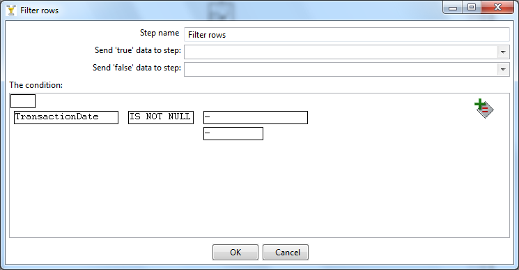
Let us now double click on the Filter step to bring up the setting dialog:

Here we specify that the filter condition is true if the TransactionDate column is not empty. Back to the canvas, we can now create 2 hops, one for the true condition that will lead to the Excel worksheet and one for the false condition which brings to the Dummy step:

We are now ready to execute the PDI Transformation. The metrics should display something like this:

Now, only 25163 rows made it to the Excel worksheet while 24837 were trashed. The resulting Excel worksheet is finally much closer to what an end user might expect:


Conclusion

In this article we have seen how mainframe data, which is by construct obscure and hardly usable by non-programmers, can be transformed into something as easy to manipulate as an Excel worksheet.

Of course, the example given remains simplistic compared to true life COBOL structures and mainframe data organizations but we have seen a small part of the PDI capabilities, some of which are pretty powerful.

Historically the type of features that you have seen in this article were only available from very expensive and proprietary products. The fact that you can now do a lot of the same things, entirely with open source software, will hopefully trigger many more opportunities to exploit the massive untapped mainframe data.

We hope that readers with mainframe background, as well as readers with open systems background, will find this useful and come out with new ideas for Open Source mainframe integration solutions.